前言

本系列文章將透過 Python 及其資料科學與機器學習生態系（Numpy、Scipy、Pandas、scikit-learn、Statsmodels、Matplotlib、Scrapy、Keras、TensorFlow 等）來系統性介紹資料科學與機器學習相關的知識。在這個單元中我們將介紹 scikit-learn 這個機器學習和資料分析神兵利器和基本的機器學習工作流程。接下來我們的範例將會使用 Ananconda、Python3 和 Jupyter Notebook 開發環境進行，若還沒安裝環境的讀者記得先行安裝。首先我們先來認識一下基本機器學習工作流程，讓讀者對於機器學習工作流有基本而全面的認識。

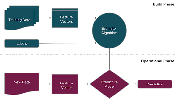
基本機器學習工作流程（Machine Learning Workflow）

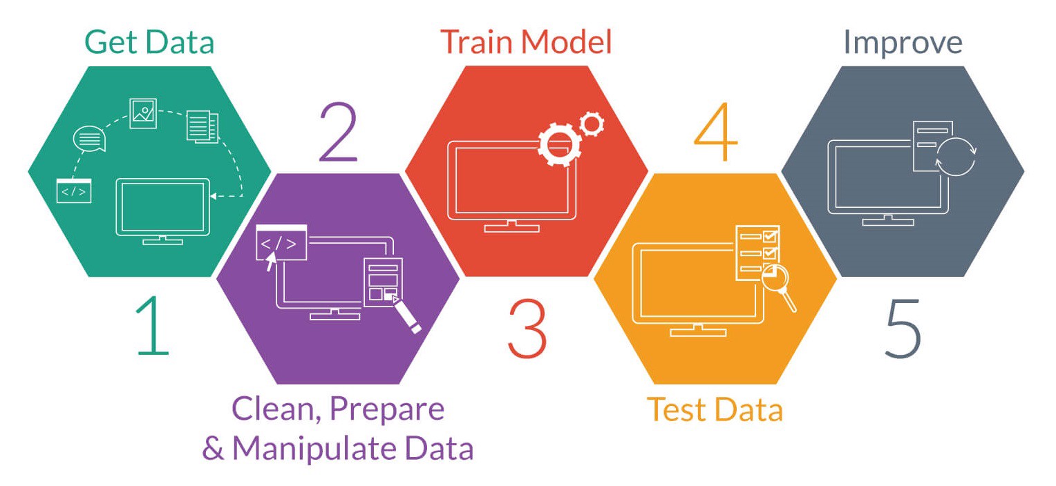
1. 明確定義問題 (Problem Definition)
2. 獲取資料與探索性資料分析 (Get Data & Exploratory Data Analysis)
3. 資料預處理與特徵工程 (Data Clean/Preprocessing & Feature Engineering)
4. 訓練模型與校調 (Model Training)
5. 模型驗證 (Model Predict & Testing)
6. 模型優化 (Model Optimization)
7. 上線運行 (Deploy Model)

明確定義問題 (Problem Definition)

明確定義問題是進行機器學習工作流的第一步。由於機器學習和一般的 Web 網頁應用程式開發比較不一樣，其需要的運算資源和時間成本比較高，若能一開始就定義好問題並將問題抽象為數學問題將有助於我們要蒐集的資料集和節省工作流程的時間。

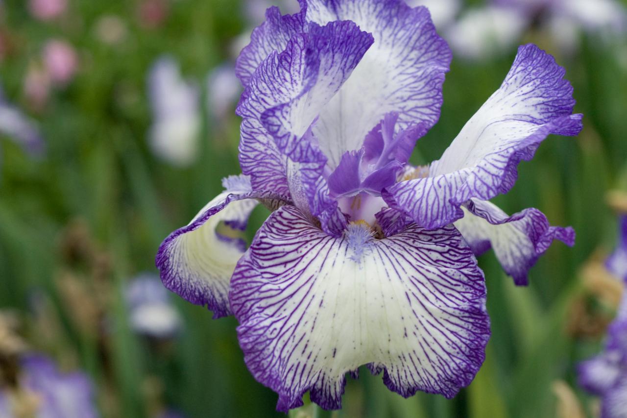
舉例來說，本篇文章範例希望預測 Iris 鳶尾花屬於哪一個類別（setosa 山鳶尾、versicolor 變色鳶尾、virginica 維吉尼亞鳶尾），這邊我們就可以決定是要進行有對應結果的監督式學習：二元分類問題（binary classification）、多類別分類問題（multi-classification）還是連續量的迴歸問題（regression），或是沒有標籤結果的非監督式學習（例如：clustering）等，我們這邊假設這是一個多類別分類問題：給定未知資料希望能預測花朵屬於哪一類。換句話說，就是說我們先定義好我們想要解決或是預測的問題，然後去蒐集對應的資料。

獲取資料與探索性資料分析 (Get Data & Exploratory Data Analysis)

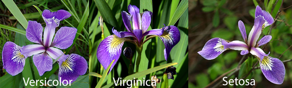
基本上資料集的完整性某種程度決定了預測結果是否能發揮模型最大功效。由於我們是教學文章，這邊我們的範例使用 scikit-learn 內建的玩具資料集 Iris（鳶尾花）的花萼、花蕊長寬進行花朵類別判別（setosa 山鳶尾、versicolor 變色鳶尾、virginica 維吉尼亞鳶尾）。在這個資料集中已經幫我們標註好每筆資料對應的類別，所以我們可以視為多類別分類問題（multi-classification）。

引入模組

# 引入 numpy、pd 和 sklearn(scikit-learn) 模組
import numpy as np
import pandas as pd
from sklearn import datasets
# 引入 train_test_split 分割方法，注意在 sklearn v0.18 後 train_test_split 從 sklearn.cross_validation 子模組搬到 sklearn.model_selection 中
from sklearn.model_selection import train_test_split
# 引入 KNeighbors 模型
from sklearn.neighbors import KNeighborsClassifier
from sklearn.svm import LinearSVC

引入資料集並進行探索性資料分析

# 引入 iris 資料集
raw_iris = datasets.load_iris()
# 探索性分析 Exploratory data analysis，了解資料集內容
# 先印出 key 值，列出有哪些值：['data', 'target', 'target_names', 'DESCR', 'feature_names']
print(raw_iris.keys())

# 印出 feature 值
print(raw_iris['data'])
# 印出目標值，分別對應的是三種花的類別：['setosa 山鳶尾' 'versicolor 變色鳶尾' 'virginica 維吉尼亞鳶尾']
print(raw_iris['target'])
# 印出目標標籤，三種花的類別：['setosa' 'versicolor' 'virginica']
print(raw_iris['target_names'])
# 印出資料集內容描述
print(raw_iris['DESCR'])
# 印出屬性名稱，['sepal length 花萼長度 (cm)', 'sepal width 花萼寬度 (cm)', 'petal length 花蕊長度 (cm)', 'petal width 花蕊寬度 (cm)']
print(raw_iris['feature_names'])

# 類別種類
print(np.unique(raw_iris.target))

dict_keys(['data', 'target', 'target_names', 'DESCR', 'feature_names'])
[[ 5.1  3.5  1.4  0.2]
 [ 4.9  3.   1.4  0.2]
 [ 4.7  3.2  1.3  0.2]
 [ 4.6  3.1  1.5  0.2]
 [ 5.   3.6  1.4  0.2]
 [ 5.4  3.9  1.7  0.4]
 [ 4.6  3.4  1.4  0.3]
 [ 5.   3.4  1.5  0.2]
 [ 4.4  2.9  1.4  0.2]
 [ 4.9  3.1  1.5  0.1]
 [ 5.4  3.7  1.5  0.2]
 [ 4.8  3.4  1.6  0.2]
 [ 4.8  3.   1.4  0.1]
 [ 4.3  3.   1.1  0.1]
 [ 5.8  4.   1.2  0.2]
 [ 5.7  4.4  1.5  0.4]
 [ 5.4  3.9  1.3  0.4]
 [ 5.1  3.5  1.4  0.3]
 [ 5.7  3.8  1.7  0.3]
 [ 5.1  3.8  1.5  0.3]
 [ 5.4  3.4  1.7  0.2]
 [ 5.1  3.7  1.5  0.4]
 [ 4.6  3.6  1.   0.2]
 [ 5.1  3.3  1.7  0.5]
 [ 4.8  3.4  1.9  0.2]
 [ 5.   3.   1.6  0.2]
 [ 5.   3.4  1.6  0.4]
 [ 5.2  3.5  1.5  0.2]
 [ 5.2  3.4  1.4  0.2]
 [ 4.7  3.2  1.6  0.2]
 [ 4.8  3.1  1.6  0.2]
 [ 5.4  3.4  1.5  0.4]
 [ 5.2  4.1  1.5  0.1]
 [ 5.5  4.2  1.4  0.2]
 [ 4.9  3.1  1.5  0.1]
 [ 5.   3.2  1.2  0.2]
 [ 5.5  3.5  1.3  0.2]
 [ 4.9  3.1  1.5  0.1]
 [ 4.4  3.   1.3  0.2]
 [ 5.1  3.4  1.5  0.2]
 [ 5.   3.5  1.3  0.3]
 [ 4.5  2.3  1.3  0.3]
 [ 4.4  3.2  1.3  0.2]
 [ 5.   3.5  1.6  0.6]
 [ 5.1  3.8  1.9  0.4]
 [ 4.8  3.   1.4  0.3]
 [ 5.1  3.8  1.6  0.2]
 [ 4.6  3.2  1.4  0.2]
 [ 5.3  3.7  1.5  0.2]
 [ 5.   3.3  1.4  0.2]
 [ 7.   3.2  4.7  1.4]
 [ 6.4  3.2  4.5  1.5]
 [ 6.9  3.1  4.9  1.5]
 [ 5.5  2.3  4.   1.3]
 [ 6.5  2.8  4.6  1.5]
 [ 5.7  2.8  4.5  1.3]
 [ 6.3  3.3  4.7  1.6]
 [ 4.9  2.4  3.3  1. ]
 [ 6.6  2.9  4.6  1.3]
 [ 5.2  2.7  3.9  1.4]
 [ 5.   2.   3.5  1. ]
 [ 5.9  3.   4.2  1.5]
 [ 6.   2.2  4.   1. ]
 [ 6.1  2.9  4.7  1.4]
 [ 5.6  2.9  3.6  1.3]
 [ 6.7  3.1  4.4  1.4]
 [ 5.6  3.   4.5  1.5]
 [ 5.8  2.7  4.1  1. ]
 [ 6.2  2.2  4.5  1.5]
 [ 5.6  2.5  3.9  1.1]
 [ 5.9  3.2  4.8  1.8]
 [ 6.1  2.8  4.   1.3]
 [ 6.3  2.5  4.9  1.5]
 [ 6.1  2.8  4.7  1.2]
 [ 6.4  2.9  4.3  1.3]
 [ 6.6  3.   4.4  1.4]
 [ 6.8  2.8  4.8  1.4]
 [ 6.7  3.   5.   1.7]
 [ 6.   2.9  4.5  1.5]
 [ 5.7  2.6  3.5  1. ]
 [ 5.5  2.4  3.8  1.1]
 [ 5.5  2.4  3.7  1. ]
 [ 5.8  2.7  3.9  1.2]
 [ 6.   2.7  5.1  1.6]
 [ 5.4  3.   4.5  1.5]
 [ 6.   3.4  4.5  1.6]
 [ 6.7  3.1  4.7  1.5]
 [ 6.3  2.3  4.4  1.3]
 [ 5.6  3.   4.1  1.3]
 [ 5.5  2.5  4.   1.3]
 [ 5.5  2.6  4.4  1.2]
 [ 6.1  3.   4.6  1.4]
 [ 5.8  2.6  4.   1.2]
 [ 5.   2.3  3.3  1. ]
 [ 5.6  2.7  4.2  1.3]
 [ 5.7  3.   4.2  1.2]
 [ 5.7  2.9  4.2  1.3]
 [ 6.2  2.9  4.3  1.3]
 [ 5.1  2.5  3.   1.1]
 [ 5.7  2.8  4.1  1.3]
 [ 6.3  3.3  6.   2.5]
 [ 5.8  2.7  5.1  1.9]
 [ 7.1  3.   5.9  2.1]
 [ 6.3  2.9  5.6  1.8]
 [ 6.5  3.   5.8  2.2]
 [ 7.6  3.   6.6  2.1]
 [ 4.9  2.5  4.5  1.7]
 [ 7.3  2.9  6.3  1.8]
 [ 6.7  2.5  5.8  1.8]
 [ 7.2  3.6  6.1  2.5]
 [ 6.5  3.2  5.1  2. ]
 [ 6.4  2.7  5.3  1.9]
 [ 6.8  3.   5.5  2.1]
 [ 5.7  2.5  5.   2. ]
 [ 5.8  2.8  5.1  2.4]
 [ 6.4  3.2  5.3  2.3]
 [ 6.5  3.   5.5  1.8]
 [ 7.7  3.8  6.7  2.2]
 [ 7.7  2.6  6.9  2.3]
 [ 6.   2.2  5.   1.5]
 [ 6.9  3.2  5.7  2.3]
 [ 5.6  2.8  4.9  2. ]
 [ 7.7  2.8  6.7  2. ]
 [ 6.3  2.7  4.9  1.8]
 [ 6.7  3.3  5.7  2.1]
 [ 7.2  3.2  6.   1.8]
 [ 6.2  2.8  4.8  1.8]
 [ 6.1  3.   4.9  1.8]
 [ 6.4  2.8  5.6  2.1]
 [ 7.2  3.   5.8  1.6]
 [ 7.4  2.8  6.1  1.9]
 [ 7.9  3.8  6.4  2. ]
 [ 6.4  2.8  5.6  2.2]
 [ 6.3  2.8  5.1  1.5]
 [ 6.1  2.6  5.6  1.4]
 [ 7.7  3.   6.1  2.3]
 [ 6.3  3.4  5.6  2.4]
 [ 6.4  3.1  5.5  1.8]
 [ 6.   3.   4.8  1.8]
 [ 6.9  3.1  5.4  2.1]
 [ 6.7  3.1  5.6  2.4]
 [ 6.9  3.1  5.1  2.3]
 [ 5.8  2.7  5.1  1.9]
 [ 6.8  3.2  5.9  2.3]
 [ 6.7  3.3  5.7  2.5]
 [ 6.7  3.   5.2  2.3]
 [ 6.3  2.5  5.   1.9]
 [ 6.5  3.   5.2  2. ]
 [ 6.2  3.4  5.4  2.3]
 [ 5.9  3.   5.1  1.8]]
[0 0 0 0 0 0 0 0 0 0 0 0 0 0 0 0 0 0 0 0 0 0 0 0 0 0 0 0 0 0 0 0 0 0 0 0 0
 0 0 0 0 0 0 0 0 0 0 0 0 0 1 1 1 1 1 1 1 1 1 1 1 1 1 1 1 1 1 1 1 1 1 1 1 1
 1 1 1 1 1 1 1 1 1 1 1 1 1 1 1 1 1 1 1 1 1 1 1 1 1 1 2 2 2 2 2 2 2 2 2 2 2
 2 2 2 2 2 2 2 2 2 2 2 2 2 2 2 2 2 2 2 2 2 2 2 2 2 2 2 2 2 2 2 2 2 2 2 2 2
 2 2]
['setosa' 'versicolor' 'virginica']
Iris Plants Database
====================

Notes
-----
Data Set Characteristics:
    :Number of Instances: 150 (50 in each of three classes)
    :Number of Attributes: 4 numeric, predictive attributes and the class
    :Attribute Information:
        - sepal length in cm
        - sepal width in cm
        - petal length in cm
        - petal width in cm
        - class:
                - Iris-Setosa
                - Iris-Versicolour
                - Iris-Virginica
    :Summary Statistics:

    ============== ==== ==== ======= ===== ====================
                    Min  Max   Mean    SD   Class Correlation
    ============== ==== ==== ======= ===== ====================
    sepal length:   4.3  7.9   5.84   0.83    0.7826
    sepal width:    2.0  4.4   3.05   0.43   -0.4194
    petal length:   1.0  6.9   3.76   1.76    0.9490  (high!)
    petal width:    0.1  2.5   1.20  0.76     0.9565  (high!)
    ============== ==== ==== ======= ===== ====================

    :Missing Attribute Values: None
    :Class Distribution: 33.3% for each of 3 classes.
    :Creator: R.A. Fisher
    :Donor: Michael Marshall (MARSHALL%PLU@io.arc.nasa.gov)
    :Date: July, 1988

This is a copy of UCI ML iris datasets.
http://archive.ics.uci.edu/ml/datasets/Iris

The famous Iris database, first used by Sir R.A Fisher

This is perhaps the best known database to be found in the
pattern recognition literature.  Fisher's paper is a classic in the field and
is referenced frequently to this day.  (See Duda & Hart, for example.)  The
data set contains 3 classes of 50 instances each, where each class refers to a
type of iris plant.  One class is linearly separable from the other 2; the
latter are NOT linearly separable from each other.

References
----------
   - Fisher,R.A. "The use of multiple measurements in taxonomic problems"
     Annual Eugenics, 7, Part II, 179-188 (1936); also in "Contributions to
     Mathematical Statistics" (John Wiley, NY, 1950).
   - Duda,R.O., & Hart,P.E. (1973) Pattern Classification and Scene Analysis.
     (Q327.D83) John Wiley & Sons.  ISBN 0-471-22361-1.  See page 218.
   - Dasarathy, B.V. (1980) "Nosing Around the Neighborhood: A New System
     Structure and Classification Rule for Recognition in Partially Exposed
     Environments".  IEEE Transactions on Pattern Analysis and Machine
     Intelligence, Vol. PAMI-2, No. 1, 67-71.
   - Gates, G.W. (1972) "The Reduced Nearest Neighbor Rule".  IEEE Transactions
     on Information Theory, May 1972, 431-433.
   - See also: 1988 MLC Proceedings, 54-64.  Cheeseman et al"s AUTOCLASS II
     conceptual clustering system finds 3 classes in the data.
   - Many, many more ...

['sepal length (cm)', 'sepal width (cm)', 'petal length (cm)', 'petal width (cm)']
[0 1 2]

資料預處理與特徵工程 (Data Clean/Preprocessing & Feature Engineering)

良好的資料輸入取決於資料預處理與特徵工程，而好的輸入將大大影響到模型是否可以發揮其理論正常水準。以下把資料轉成 DataFrame 格式方便進行操作。由於這邊的資料集已經是相當完整的資料集，所以我們這邊就不用特別進行資料預處理和特徵工程的部份，然而在真實世界中，真正在進行機器學習工作流程的時候資料預處理往往是最花時間的部份。同時為了方便模型的校調，我們這邊把資料集分為 70% 訓練資料，30% 驗證資料。

# 將資料轉為 pandas DataFrame
# data 為觀察目標變數
df_X = pd.DataFrame(raw_iris.data)
# target 為預測變數
df_y = pd.DataFrame(raw_iris.target)

# 將資料切分為 training data 和 testing data，其中 random_state 若設為 0 或不設則即便實例不同但因種子相同產生同樣隨機編號，若設為 1 則每次隨機產生不同編號
# test_size 為切分 training data 和 testing data 的比例
X_train, X_test, y_train, y_test = train_test_split(df_X, df_y, test_size=0.3)

# 印出所有資料集筆數
print(len(df_y))

150

# 印出切分 y_train 的數量為所有資料集的 70%，共 105 筆
print(y_train)
print(len(y_train))

     0
39   0
106  2
99   1
0    0
16   0
118  2
80   1
29   0
11   0
104  2
100  2
72   1
108  2
42   0
20   0
31   0
115  2
111  2
89   1
83   1
130  2
41   0
66   1
120  2
113  2
6    0
126  2
62   1
23   0
97   1
..  ..
10   0
76   1
129  2
144  2
137  2
12   0
79   1
123  2
127  2
36   0
74   1
37   0
131  2
110  2
22   0
32   0
147  2
134  2
102  2
75   1
88   1
148  2
33   0
56   1
28   0
90   1
82   1
25   0
121  2
13   0

[105 rows x 1 columns]
105

# 印出切分的 y_test 資料為所有資料集的 30%，共 45 筆
print(y_test)
print(len(y_test))

     0
102  2
53   1
143  2
70   1
61   1
67   1
24   0
124  2
36   0
92   1
114  2
31   0
120  2
87   1
74   1
47   0
69   1
56   1
93   1
16   0
144  2
133  2
29   0
57   1
116  2
50   1
86   1
44   0
3    0
21   0
82   1
99   1
134  2
111  2
135  2
4    0
2    0
91   1
85   1
122  2
127  2
11   0
27   0
79   1
51   1
45

訓練模型與校調 (Model Training)

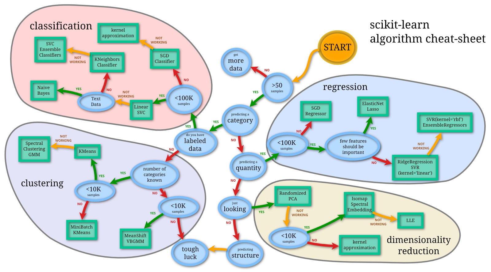
上面是 scikit-learn 提供的演算法 cheat-sheet，當你面對琳琅滿目的模型一開始不知道要選擇什麼的話可以按圖索驥參考，另外這邊提供大圖支援連結。

這邊我們參考上圖來選擇適合模型：

1. 樣本資料是否大於 50 筆：範例資料集總共有 150 筆資料，大於 50
2. 是否為分類問題：Iris 花朵類別預測是多類別分類問題
3. 是否有標籤好的資料：已經有 label 資料
4. 樣本資料是否小於 100K：資料小於 100K
5. 選擇 Linear SVC 模型（第一個選擇的模型）
6. 是否是文字資料：不是
7. 選擇 KNeighborsClassifier 模型（第二個選擇的模型）
8. 後續優化 / SVC / Ensemble

# 初始化 LinearSVC 實例
lin_clf = LinearSVC()
# 使用 fit 來建置模型，其參數接收 training data matrix, testing data array，所以進行 y_train.values.ravel() Data Frame 轉換
lin_clf.fit(X_train, y_train.values.ravel())

LinearSVC(C=1.0, class_weight=None, dual=True, fit_intercept=True,
     intercept_scaling=1, loss='squared_hinge', max_iter=1000,
     multi_class='ovr', penalty='l2', random_state=None, tol=0.0001,
     verbose=0)

# 初始化 KNeighborsClassifier 實例
knn = KNeighborsClassifier()

# 使用 fit 來建置模型，其參數接收 training data matrix, testing data array，所以進行 y_train.values.ravel() 轉換
knn.fit(X_train, y_train.values.ravel())

KNeighborsClassifier(algorithm='auto', leaf_size=30, metric='minkowski',
           metric_params=None, n_jobs=1, n_neighbors=5, p=2,
           weights='uniform')

模型驗證 (Model Predict & Testing)

監督式學習的分類問題通常會分為訓練模型和驗證模型，這邊我們使用 predict 去產生對應的目標值，此時和正確答案（已經標籤好的目標值）比較可以知道模型預測的正確率。我們可以看到 KNeighborsClassifier 在正確率（accuracy）表現上相對比較好一點（0.98 比 0.93）。

# 使用 X_test 來預測結果
print(lin_clf.predict(X_test))

[1 1 0 2 1 2 0 1 1 2 2 1 0 2 0 0 2 1 2 0 0 1 2 0 2 1 2 0 0 0 1 0 2 1 1 0 0
 0 1 0 1 2 2 1 1]

# 印出預測準確率
print(lin_clf.score(X_test, y_test))

0.933333333333

# 使用 X_test 來預測結果
print(knn.predict(X_test))

[1 1 0 1 1 2 0 1 1 2 2 1 0 2 0 0 2 1 2 0 0 1 2 0 2 1 2 0 0 0 1 0 1 1 1 0 0
 0 1 0 1 2 2 1 1]

# 印出 testing data 預測標籤機率
print(knn.predict_proba(X_test))

[[ 0.   1.   0. ]
 [ 0.   1.   0. ]
 [ 1.   0.   0. ]
 [ 0.   0.8  0.2]
 [ 0.   1.   0. ]
 [ 0.   0.   1. ]
 [ 1.   0.   0. ]
 [ 0.   1.   0. ]
 [ 0.   1.   0. ]
 [ 0.   0.   1. ]
 [ 0.   0.   1. ]
 [ 0.   1.   0. ]
 [ 1.   0.   0. ]
 [ 0.   0.   1. ]
 [ 1.   0.   0. ]
 [ 1.   0.   0. ]
 [ 0.   0.   1. ]
 [ 0.   1.   0. ]
 [ 0.   0.   1. ]
 [ 1.   0.   0. ]
 [ 1.   0.   0. ]
 [ 0.   1.   0. ]
 [ 0.   0.   1. ]
 [ 1.   0.   0. ]
 [ 0.   0.2  0.8]
 [ 0.   1.   0. ]
 [ 0.   0.   1. ]
 [ 1.   0.   0. ]
 [ 1.   0.   0. ]
 [ 1.   0.   0. ]
 [ 0.   1.   0. ]
 [ 1.   0.   0. ]
 [ 0.   1.   0. ]
 [ 0.   1.   0. ]
 [ 0.   1.   0. ]
 [ 1.   0.   0. ]
 [ 1.   0.   0. ]
 [ 1.   0.   0. ]
 [ 0.   0.6  0.4]
 [ 1.   0.   0. ]
 [ 0.   1.   0. ]
 [ 0.   0.   1. ]
 [ 0.   0.   1. ]
 [ 0.   1.   0. ]
 [ 0.   1.   0. ]]

# 印出預測準確率
print(knn.score(X_test, y_test))

0.977777777778

模型優化 (Model Optimization)

由於本文是簡易範例，這邊就沒有示範如何進行模型優化（這邊可以嘗試使用 SVC 和 Ensemble 方法）。不過一般來說在分類模型優化上，讓模型預測表現的更好的方法大約有幾種：

1. 特徵工程：選擇更適合特徵值或是更好的資料清理，某種程度上很需要專業知識的協助（domain konwledge）去發現和整合出更好的 feature
2. 調整模型參數：調整模型的參數
3. 模型融合：結合幾個弱分類器結果來變成強的分類器

上線運行 (Deploy Model)

當模型優化完畢就可以進行上線運行，其中 Python 比 R 更具優勢的地方，那就是 Python 很容易跟現有的系統進行整合，Python 也有許多好用的 Web 框架可以使用，也因為 Python 是膠水語言，若要進行效能優化也可以很容易呼叫 C/C++ 進行操作，提昇執行效能。

總結

以上用一個簡單的範例介紹了 Python 機器學習套件 Scikit Learn 的基本功能和機器學習整個基本 Workflow。由於是基礎範例所以省略一些比較繁瑣的資料處理部分，事實上，真實世界資料大多是非結構化資料的髒資料，而資料分析的過程往往需要花上許多時間進行資料預處理和資料清理上。接下來我們將介紹其他 Python 資料科學和機器學習生態系和相關工具。

延伸閱讀

1. 机器学习实战 之 kNN 分类
2. Machine Learning Workflow
3. Kaggle机器学习之模型融合（stacking）心得
4. Python 資料視覺化
5. Train & Predict workflow
6. Sample Classification Pipeline workflow
7. 【机器学习】模型融合方法概述

關於作者：
@kdchang 文藝型開發者，夢想是做出人們想用的產品和辦一所心目中理想的學校。A Starter, Software Engineer & Maker. JavaScript, Python & Arduino/Android lover. Interested in Internet, AI and Blockchain.:)

（image via medium、mapr、silvrback、camo、scipy、mirlab、concreteinteractive、sndimg）